Tutorial: Tree-based and ensemble models in Python (ANSWERS)¶

This is not a standalone tutorial, as most of the theory and important questions are asked in the main tutorial in R. The second tutorial serves the purpose of helping you make your own tree-based and enseble models in Python. I expect that you have already covered the video lectures and the main tutorial in R by now. So I assume that you already know what you are doing, you just don’t know how to code it in Python yet. If R tutorial provides more assistance in digesting the material, this tutorial in Python pushes you to be more independent, with minimum hints. (I used these notebooks to prepare this tutorial: 1, 2 3)

We keep on working with the same COMPAS dataset, and we will use sklearn library.

# Import the usual libraries
import sys
import sklearn
import numpy as np
import pandas as pd
import os

Load data and split it in train and test sets¶

Let’s load the sample of COMPAS data we used in the previous tutorial. For your convenience, I already transformed all factor variables into dummy variables using model.matrix() function in R and saved it on github as a csv file. So you can directly access the data using the link below.

data_location = "https://raw.githubusercontent.com/madina-k/DSE2021_tutorials/main/tutorial_trees/data/compas_sample500matrix.csv"
data = pd.read_csv(data_location)
data.head()

	Two_yr_Recidivismyes	Number_of_Priors	Age_Above_FourtyFiveyes	Age_Below_TwentyFiveyes	FemaleMale	Misdemeanoryes	ethnicityCaucasian
0	1	-0.012530	0	1	0	1	1
1	1	-0.400115	0	1	1	1	0
2	1	0.701857	1	0	1	1	0
3	0	-0.930922	0	0	1	0	1
4	1	-0.545324	0	1	1	1	0

Use train_test_split command from sklearn.model_selection to split the data into four objects: X_train, X_test, y_train, y_test

from sklearn.model_selection import train_test_split


y = data.pop('Two_yr_Recidivismyes').values
X = data
X_train, X_test, y_train, y_test = train_test_split(X, y, random_state=1)

Decision Tree¶

Train a decision tree using DecisionTreeClassifier class from sklearn.tree. Look at the documentation here and fit a decision tree using Gini node impurity measure, with minimum 25 observations in each leaf, and the maximum tree depth of 3.

from sklearn.tree import DecisionTreeClassifier

tree_clf = DecisionTreeClassifier(min_samples_leaf = 25, max_depth=4)
tree_clf.fit(X,y)

DecisionTreeClassifier(class_weight=None, criterion='gini', max_depth=4,
                       max_features=None, max_leaf_nodes=None,
                       min_impurity_decrease=0.0, min_impurity_split=None,
                       min_samples_leaf=25, min_samples_split=2,
                       min_weight_fraction_leaf=0.0, presort=False,
                       random_state=None, splitter='best')

And visualize the resulting tree using plot_tree from sklearn.tree. See documentation here. Don’t forget to tell the names of the features and class names, set the font size to 14.

from sklearn.tree import plot_tree
import matplotlib.pyplot as plt

plt.figure(figsize=(18,18))  # set plot size (denoted in inches)
plot_tree(tree_clf, feature_names=X.columns, class_names=['No', 'Yes'],fontsize=14 )
plt.show()

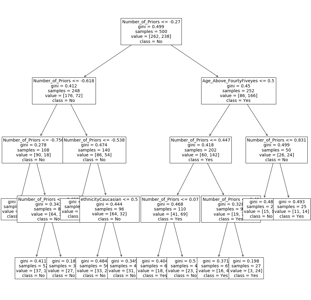
This is some bushy tree but we do not have a way to prune it in an automated way with sklearn. If you really want to prune this tree, look how it can be done in this blog.

Finally, let’s check it’s out-of-sample accuracy with accuracy_score function from sklearn.metrics. Read the documentation here.

from sklearn.metrics import accuracy_score

y_pred_tree = tree_clf.predict(X_test)
print(accuracy_score(y_test, y_pred_tree))

0.728

Bagging¶

Now it’s time for some bagging! Use BaggingClassifier from sklearn.ensemble. See documentation here. Create a new tree object which allows to grow a tree of maximum depth of 2 and put that classifier inside the BaggingClassifier. Ask to bag over 500 trees with maximum samples of 100 observations with bootstrapping. Print the accuracy score.

from sklearn.ensemble import BaggingClassifier

tree_clf_forbagging = DecisionTreeClassifier(max_depth=2)

bag_clf = BaggingClassifier(
    tree_clf_forbagging, n_estimators=500,
    max_samples=100, bootstrap=True)
bag_clf.fit(X_train, y_train)
y_pred_bag = bag_clf.predict(X_test)
print(accuracy_score(y_test, y_pred_bag))

0.72

Random Forest¶

Now, let’s use RandomForestClassifier from sklearn.ensemble. See documentation here. Create a random forest of 500 trees, where each tree has a maximum depth of 2. Print the accuracy score for the test sample.

from sklearn.ensemble import RandomForestClassifier

rf_clf = RandomForestClassifier(n_estimators=500, max_depth=2)
rf_clf.fit(X_train, y_train)

y_pred_rf = rf_clf.predict(X_test)

print(accuracy_score(y_test, y_pred_rf))

0.696

Check for the importance of each feature, using feature_importances_ property of the classifier. (For example, see this page)

for name, score in zip(list(data.columns), rnd_clf.feature_importances_):
    print(name,score)

Number_of_Priors 0.5951675288832771
Age_Above_FourtyFiveyes 0.15327959016558776
Age_Below_TwentyFiveyes 0.04963856624481278
FemaleMale 0.06136793924146804
Misdemeanoryes 0.07341448602922451
ethnicityCaucasian 0.06713188943562985

Boosting with Gradient Boosting¶

There are several different ways to boost trees (e.g., XGBoost library or AdaBoostClaasifier from sklearn). In this tutorial, I would ask you to train a GradientBoostingClassifier from sklearn.ensemble. See the documentation here. Make 300 trees with the maximum depth of 2. Set learning rate at 0.01.

Then use the staged_predict method to predict the target variable at each stage of boosting (1 tree only, 2 trees together, 3 trees, and so on) using the test X. Get the mean squared error using the mean_squared_error wrapper from sklearn.ensemble. See the documentation here. And find the number of trees that minimize the MSE on the test sample.

from sklearn.metrics import mean_squared_error
from sklearn.ensemble import GradientBoostingClassifier

gbc_clf = GradientBoostingClassifier(max_depth=2, n_estimators=300, learning_rate=0.01)
gbc_clf.fit(X_train, y_train)

errors = [mean_squared_error(y_test, y_pred)
          for y_pred in gbc_clf.staged_predict(X_test)]

min_error = np.min(errors)
print(min_error)


optimal_n_trees = np.argmin(errors) + 1
print(optimal_n_trees)

0.304
26

Train the Gradient boosting classifier model with the optimal number of trees and and get the accuracy score.

gbc_best = GradientBoostingClassifier(max_depth=2, n_estimators=optimal_n_trees, learning_rate=0.01)
gbc_best.fit(X_train, y_train)

y_pred_gbcbest = gbc_best.predict(X_test)
print(accuracy_score(y_test, y_pred_gbrtbest))

0.696

Voting classifier¶

Finally we will try to combine all the other models under one Ensemble model.

Import VotingClassifier from sklearn.ensemble.

We will also import Logistic Regression and Support Vector Machine.

from sklearn.ensemble import VotingClassifier
from sklearn.linear_model import LogisticRegression
from sklearn.svm import SVC

log_clf = LogisticRegression(solver='lbfgs')
svm_clf = SVC(probability=True, gamma='scale')

Now put all different classifiers to be combined within the voting classifier and compare accuracy scores across different classifiers:

voting_clf = VotingClassifier(
    estimators = [('lr', log_clf), # Logistic classifier
                  ('rf', rf_clf),  # Random forest classifier
                  ('svm', svm_clf), # SVM classifier
                  ('bag', bag_clf), # Bagging classifier
                  ('gbrt', gbc_best)],  # Boosting classifier
    voting ='hard')

for clf in (tree_clf,log_clf, rf_clf, svm_clf, bag_clf, gbc_best, voting_clf):
    clf.fit(X_train, y_train)
    y_pred = clf.predict(X_test)
    print(clf.__class__.__name__, accuracy_score(y_test, y_pred))

DecisionTreeClassifier 0.624
LogisticRegression 0.656
RandomForestClassifier 0.696
SVC 0.688
BaggingClassifier 0.728
GradientBoostingClassifier 0.696
VotingClassifier 0.72

Data Science for Economics Tilburg U 2021